
{(0, 3), (10, 4), (20, 5), (30, 0), (40, 1), (50, 2), (59, 3)} interpolated to 60 bins using the spline.This manuscript (permalink) was automatically generated from slochower/nonequilibrium-barrier@d905240 on May 11, 2018.
What is the relationship between the “conventional” stall force results and the forces on infinitely high barriers? It would be nice if we could find a concrete relationship, but I’m not convinced one exists. Discussion
Should we test our “pressure” method of computing the force with a numerical example? I think the way to do this would be to set up a motor model with a very large number of bins (e.g. 1000). Discussion
Our motor models so far assume a catalytic rate constant that is uniform in dihedral \(\phi\). How would the present results change if \(k_\text{cat} > 0\) were focused in some key part of the cycle? Would this get rid of zero-torque locations? Discussion
The instantaneous force on a soft wall due to the diffusion of a particle at position \(x\) in a potential \(E(x)\) is \(F(x) = \partial E(x) / \partial x\). The mean force is then \[ \langle F \rangle = \frac{\int_0^\infty \partial E(x)/ \partial x \exp(-\beta E(x)) \, \mathrm{d}x}{L + \int_0^\infty \exp(-\beta E(x)) \,\mathrm{d}x}, \] assuming \(E(x) = 0\) for \(x < 0\) and a flat potential from \(x = -L\) to \(x = 0\). The numerator integrates to \(k_{B}T\), and in the limit \(L \rightarrow \infty\), the mean force becomes \[ \langle F \rangle = \frac{k_{B}T}{L}. \] For \(N\) non-interacting particles, we can write \[ \lim_{L \rightarrow \infty} \langle F \rangle = \frac{Nk_{B}T}{L}. \]
From this, we reasoned that the force on a barrier at position \(i\) should go as \[ F_{i} \propto p_{i} kT, \] for population \(i\) in bin \(i\). Then we claim the net force on the barrier is something like \(F_{i} = F_{i-1} - F_{i+1}\) depending on whatever convention we pick for the sign. Later, we agreed (email on June 22, 2017) it’s correct to divide the population by the bin width, or else the force would increase just from using larger bins. Thus, we concluded the force should go as \[ F_{i} = \frac{RT}{L} p_{i-1} - \frac{RT}{L} p_{i+1} = \frac{RT}{L} (p_{i-1} - p_{i+1}) = \frac{RT N_\text{bins}}{2 \pi} (p_{i-1} - p_{i+1}). \](1)
It would be nice to be able to design – or suggest how to design – a molecular motor for specific properties: speed, force, torque, gearing, ability to work against a load, resistance to being forced backwards, or something else. To that end, we set out to explore the relationship between the shape of the potential energy surfaces and these properties.
{(0, 3), (10, 4), (20, 5), (30, 0), (40, 1), (50, 2), (59, 3)} interpolated to 60 bins using the spline.
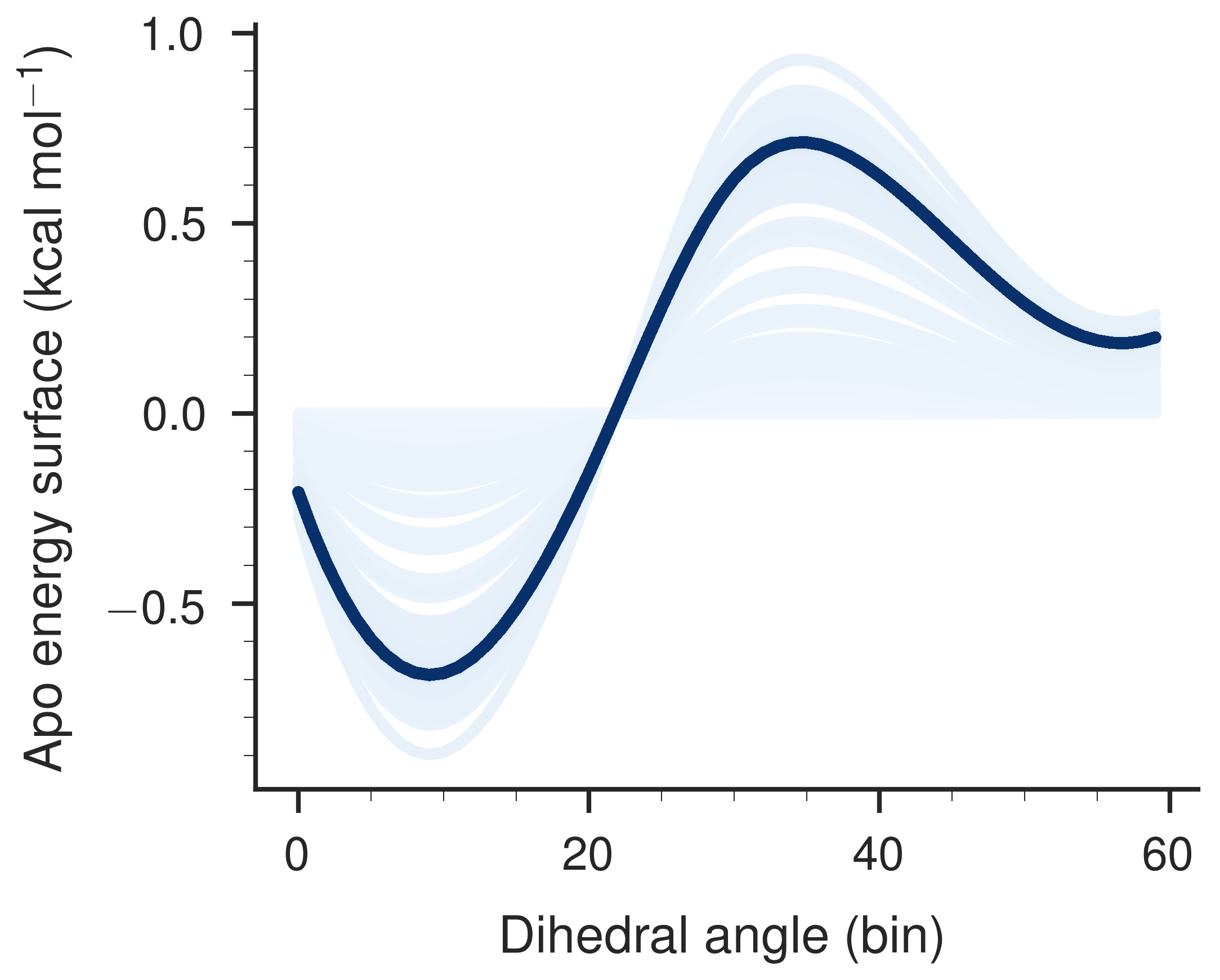
To start, let’s begin with a fixed bound energy surface created by smoothing a sawtooth with seven spline points (Figure 2). I couldn’t find a way to spline across the periodic boundary, so the curve looks a little wonkier than expected. My first attempt was to use a downhill simplex method (Nelder-Mead) to optimize the apo surface for maximal flux. The algorithm begins with an initial guess of a flat apo surface. The results are not completely deterministic, even with with setting np.random.seed(42), and I don’t understand that. After 100 loops of the same optimization, using the same initial conditions and random seed, the number of function evaluations in each optimization bounces between around 1400 and around 500! The non-repeatability of the optimization is repeatable itself, however! Upon running a further 100 loops on a different day, I observed the same bouncing between 1400 and 500 iterations. I could look into this further, but I haven’t. It may have to do with the interpolation.


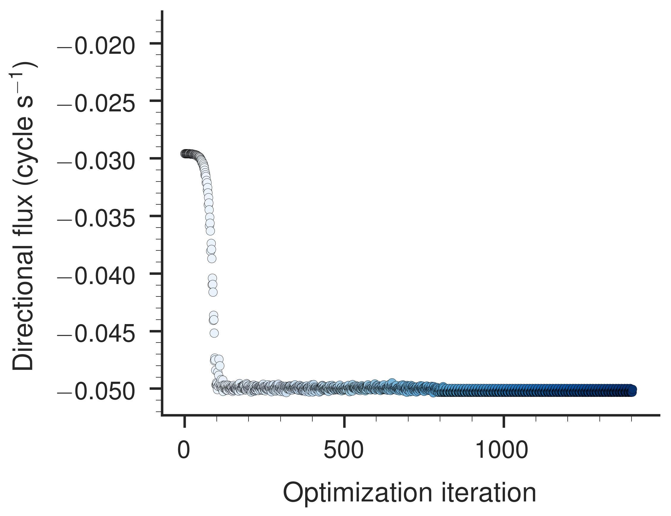
After 1403 iterations, Nelder-Mead optimization results in the surface shown in Figure 5. Each blue line is an iteration of the optimization. Lighter colors correspond to earlier iterations. The final surface is darker because many lines are overlaid. I have not implemented bounds on the optimization because Nelder-Mead does not allow bounds, as far as I know. I’ll return to the idea of using bounds a little later. The result of this optimization is that the flux starts near \(0\) (although not exactly at zero, curiously) and drops to \(-0.050 \,\text{cycle s}^{-1}\) quickly and stays there.
COBYLA and Powell’s method result in better optimization than simplex downhill. After 269 iterations, COBYLA approaches flux of more than \(-250 \,\text{cycle s}^{-1}\), with the flux beginning to decrease after just a few iterations. The iterations of COBYLA look like they are refining a single landscape, instead of jumping around. Powell’s method does well, too, although it occasionally jumps back to near zero flux after finding a high value.
Taken together, the fixed bound surface and the COBYLA-optimized apo surface are shown below.
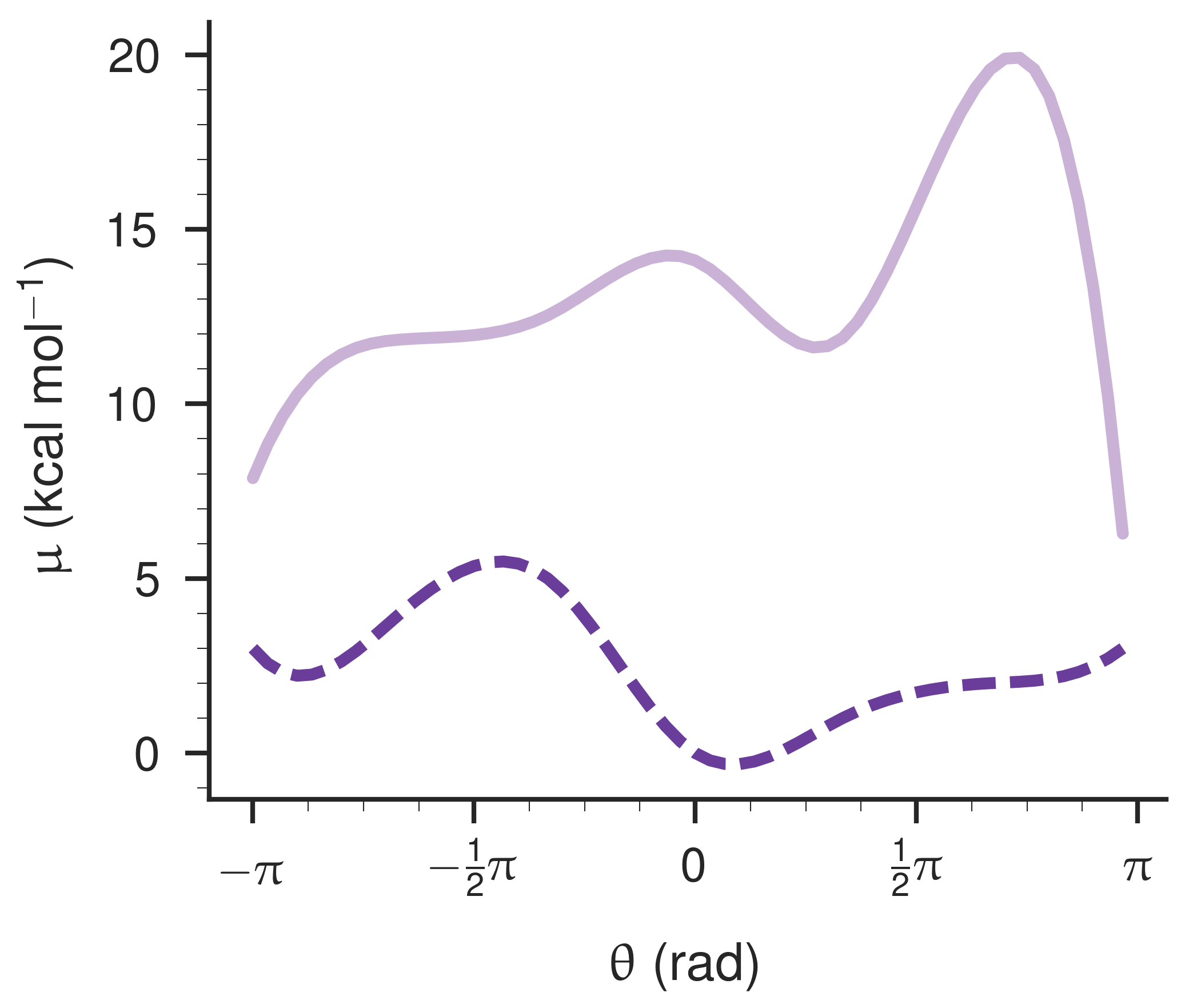
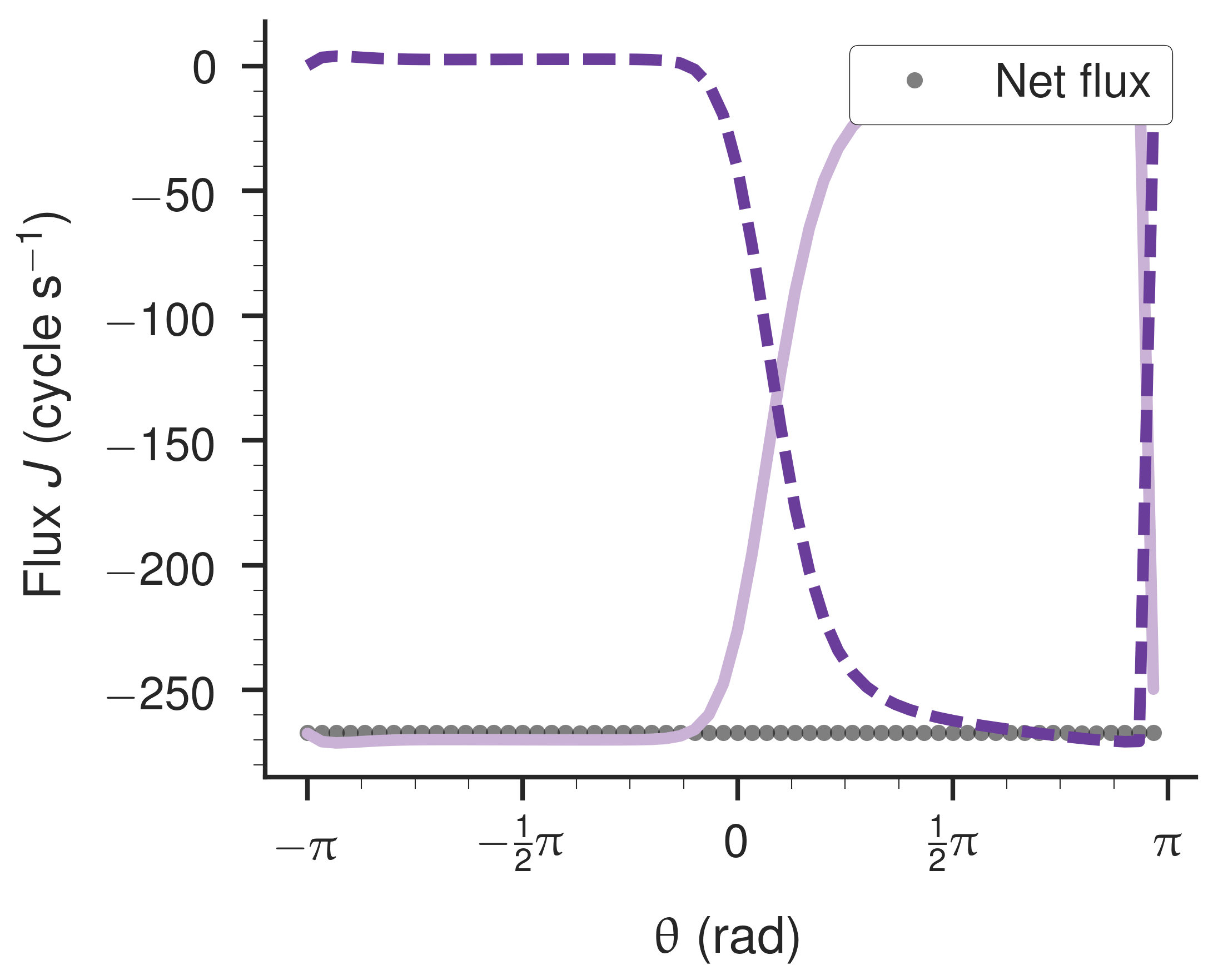
Curiously, the flux is mostly zero across the
COBYLA in particular handles the bounds and produces highly optimized surfaces after just a few iterations.